Do you ever wonder why your computer doesn't get tired when you ask it to do lots of things? It's because of something called "time complexity," which is like telling your computer how fast or slow it should work.

Time complexity measures how the runtime of an algorithm grows as the input size increases. It quantifies the worst-case performance and helps us compare algorithms in terms of efficiency.

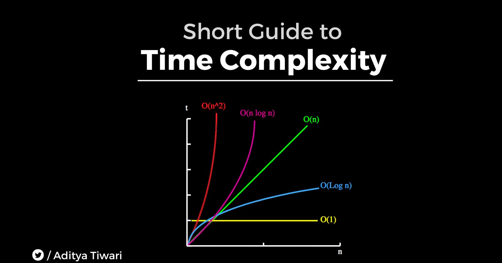
Express time complexity using Big O notation, like O(1), O(log n), O(n), O(n log n), O(n^2), etc. This notation describes the upper bound of an algorithm's runtime.

Wait, What is Big O notation?

Big O notation is a way to describe the upper bound or worst-case performance of an algorithm in computer science. It's a shorthand method to express how the runtime or space requirements of an algorithm grow relative to the size of the input. Here's what you need to know about it:

Expressing Efficiency: Big O notation helps us understand how efficient an algorithm is by focusing on its scaling behavior as the input size increases. It provides a high-level view of an algorithm's performance.

Upper Bound: Big O notation describes the upper limit of an algorithm's resource usage (usually time or space). It tells us that an algorithm will not perform worse than this bound, even in the worst-case scenario.

Big O notation is like a handy speedometer for algorithms. It helps us understand how fast or slow an algorithm will be when we throw big or small problems at it, making it a crucial concept for anyone working with computers and programming.

Most Common Time Complexities

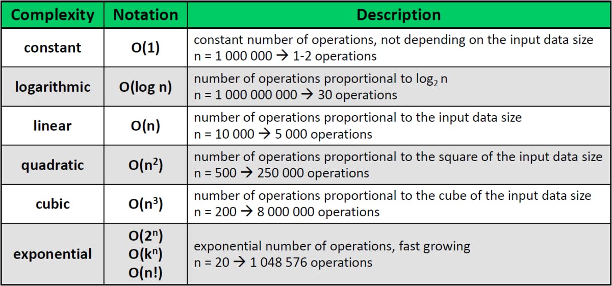
1. O(1) Constant Time

• In this time complexity, the algorithm takes the same amount of time to complete regardless of the input's size.

• Suppose you are accessing an element in an array or list by its index. It doesn't matter if the array has 10 or 10,000 items; it takes roughly the same time.

• In this example, regardless of the size of the list, the function accesses the first element directly, taking constant time.

•     def constant_time_example(my_list):
          return my_list[0]
  
      my_list = [1, 2, 3, 4, 5]
      result = constant_time_example(my_list)
      print(result)  # Output: 1
  

2. O(log n) - Logarithmic Time:

• Algorithms with O(log n) time complexity typically divide the input into smaller portions at each step.

• Imagine you have a phone book with 1,000 pages, and you're looking for a name. You don't start at page 1 and flip through every page. Instead, you open the book in the middle, check if the name is in the left or right half, and repeat this process, dividing the search space in half each ti

  me.

• Example: Binary search in a sorted list. With each step, you eliminate half of the remaining options.

• Code Example : Here, we use binary search to find an item in a sorted list. It's like a smart way of looking things up, quickly narrowing down the search space by half each time.

•     def binary_search(arr, target):
          left, right = 0, len(arr) - 1
          while left <= right:
              mid = left + (right - left) // 2
              if arr[mid] == target:
                  return mid
              elif arr[mid] < target:
                  left = mid + 1
              else:
                  right = mid - 1
          return -1
  
      my_list = [1, 2, 3, 4, 5, 6, 7, 8, 9, 10]
      target = 5
      result = binary_search(my_list, target)
      print(result)  # Output: 4 (index of the target value)
  

3. O(n) Linear Time

• Algorithms with O(n) time complexity have a runtime that's directly proportional to the size of the input.

• Think of O(n) as a line of cars waiting at a toll booth. If there are 10 cars, it takes a certain amount of time to process them. If there are 100 cars, it takes roughly 10 times longer.

• Example: Checking each item in a list to find a specific value. If the list has 10 items, you may need to check all 10.

• Code Example : This function finds the maximum value in a list by checking each element one by one. It takes longer if the list has more items.

•   def find_max(arr):
        max_val = arr[0]
        for num in arr:
            if num > max_val:
                max_val = num
        return max_val
  
    my_list = [7, 2, 9, 4, 1, 8]
    result = find_max(my_list)
    print(result)  # Output: 9 (maximum value in the list)
  

4. O(n logn) Quasilinear Time:

• It's faster than quadratic time complexities (e.g., O(n^2)) but slower than linear time complexities (e.g., O(n)).

• As the input size increases, the runtime grows slightly faster than linear but significantly slower than quadratic.

• This time complexity is common in efficient sorting algorithms like merge sort and heapsort.

• Code Example : The merge sort algorithm efficiently sorts a list by repeatedly dividing it into smaller pieces, sorting them, and then combining them. It's faster than some other sorting methods but not as quick as constant or logarithmic time.

def merge_sort(arr):
    if len(arr) <= 1:
        return arr

    mid = len(arr) // 2
    left_half = arr[:mid]
    right_half = arr[mid:]

    left_half = merge_sort(left_half)
    right_half = merge_sort(right_half)

    return merge(left_half, right_half)

def merge(left, right):
    result = []
    i = j = 0

    while i < len(left) and j < len(right):
        if left[i] < right[j]:
            result.append(left[i])
            i += 1
        else:
            result.append(right[j])
            j += 1

    result.extend(left[i:])
    result.extend(right[j:])
    return result

my_list = [3, 1, 4, 1, 5, 9, 2, 6, 5, 3, 5]
sorted_list = merge_sort(my_list)
print(sorted_list)  # Output: [1, 1, 2, 3, 3, 4, 5, 5, 5, 6, 9]

5. O(n^2) and Beyond - Quadratic Time and Higher

• Algorithms with O(n^2) time complexity and higher grow rapidly with the size of the input.

• These algorithms become impractical for large inputs; their runtime can quickly become unmanageable.

• Imagine you're organizing a group photo, and everyone needs to shake hands with everyone else. If there are 10 people, that's 10 handshakes. But if there are 100 people, it's 10,000 handshakes - much more work.

• Bubble sort is an example of an O(n^2) sorting algorithm. It repeatedly compares and swaps elements in nested loops, which becomes slower as the list gets larger.

•     def bubble_sort(arr):
          n = len(arr)
          for i in range(n):
              for j in range(0, n-i-1):
                  if arr[j] > arr[j+1]:
                      arr[j], arr[j+1] = arr[j+1], arr[j]
  
      my_list = [64, 34, 25, 12, 22, 11, 90]
      bubble_sort(my_list)
      print(my_list)  # Output: [11, 12, 22, 25, 34, 64, 90]
  

Short Summary

• O(1) is super fast and doesn't depend on the input size.

• O(log n) is also fast; it divides the problem in half with each step.

• O(n) grows linearly with the input size.

• O(n log n) is efficient for sorting and grows a bit faster than linear but not as bad as quadratic.

• O(n^2) and higher are less efficient and can become very slow for large inputs.

  

That's all for today's blog on Time Complexity. Hope it helped you. I tried to keep it as easy as possible.

Any doubts or wanna connect with me? Instagram , Twitter , Linkedin